What is a covariance matrix? A covariance matrix is an essential part of the Kalman Filter output. If you have tried to learn about it by working through the expected value proof, you probably are still having a hard time understanding it. Why? Because the covariance matrix is best understood by visualizing it as an error ellipse or error ellipsoid. But before we do that, lets quickly go over covariance of a matrix in super simple terms and then we’ll move on to pictures!
Covariance of a Matrix Explained Simply
A matrix is like a grid made up of rows and columns, kind of like a spreadsheet. Each number in the matrix is called an element. Now, the covariance of a matrix is a way to measure how much two things in the matrix change together.
Let’s imagine we have a matrix that represents the position and velocity of a moving object. The rows might represent different times, and the columns might represent the position and velocity of the object at that time. The position might be measured in meters, and the velocity might be measured in meters per second.
Now, let’s say we want to know how much the object’s position and velocity are related. If the covariance of the matrix is positive, that means that as the object’s position increases, its velocity tends to increase as well. If the covariance is negative, that means that as the object’s position increases, its velocity tends to decrease.
The covariance of a matrix can be used in lots of different ways, like in physics or engineering. It helps us understand how different variables are related to each other. For a Kalman Filter, both the input and output could have covariance matrices. So let us look at these visually to build on our understanding.
Before we jump into error ellipses, let us remind ourselves of what it means to have a data set that is normally distributed or gaussian distributed.
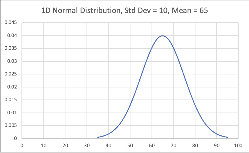
1D Normal Distribution
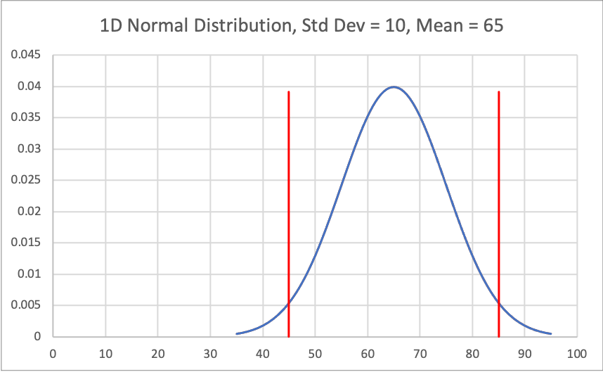
Figure 1 shows the normal distribution or gaussian distribution of a variable with a mean of 65 and standard deviation of 10. With that information, we can create Figure 2 which shows a 95% confidence interval for that same variable. 95% confidence interval is contained by 2 standard deviations.
This means that 95% of the samples taken from this particular normal distribution will be contained in the confidence interval denoted by the two red interval boundaries
Okay great, now that we agree on what a normally distributed data set looks like and how we can use a confidence interval to bound our expectations, let us consider a covariance matrix.
The covariance matrix used in the Kalman Filter represents the error of a multidimensional gaussian distributed data set. So, instead of a 1D distribution, let us consider a 2D distribution.
When you have multiple dimensions, you can no longer represent the mean as a single value with a bell curve like Figure 1 and Figure 2. With multiple dimensions, parameters can be correlated. The covariance matrix is where this information is captured.
Using the covariance matrix, we can draw confidence ellipses around 2D data sets in a comparable way that we drew confidence bounds around a single parameter. Let us now look at ellipses created from 2D covariance matrices.
2 Simple Covariance Matrices
Let us look at two different covariance matrices, one without correlation between the two parameters and one with correlation between the two parameters.
Before we do that, let us consider the unique properties of an ellipse that will allow us to visualize it i.e. center, major axis, minor axis, and angle of rotation. (Note, there are other properties of an ellipse that can define its shape (e.g. vertex and foci), but we are not going to use those)
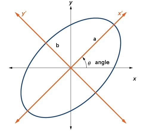
Figure 3 (above) shows a rotated ellipse about the origin of an x-y coordinate frame. The center of this ellipse is at coordinates (0,0). The major axis of an ellipse is the larger of the two primary axes and minor axis of an ellipse is the smaller of the two primary axes. These axes are perpendicular to each other and intersect at the center point. The major axis for the ellipse in Figure 3 is equal to 2a and the minor axis is equal to 2b. Therefore, the semi-major axis is equal to a and the semi-minor axis is equal to b. The major and minor axes are aligned with x’ and y’ coordinate frame. The x’-y’ coordinate frame can be thought of as a the same as x-y coordinate frame but rotated at the center by a rotation angle of theta.
So, now all we need to do is understand how a covariance matrix specifies the major axis, minor axis, and angle of rotation of an ellipse in order to visualize it.
Covariance Matrix without Correlation between X and Y
Figure 4 (below) represents a covariance matrix, D, that is specified in Figure 5 (below). The blue ellipse is based on a 1-sigma or 67% confidence interval while the orange ellipse is based on a 2-sigma or 95% confidence interval.
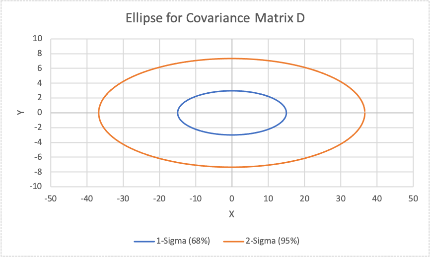
In Figure 5, you will see the covariance matrix, D, that was used to create these error ellipses. Two key takeaways from these figures are:
- The variance terms align with magnitude of the semi-major and semi-minor axes or the spread of the data i.e. a and b.
- The cross terms (i.e. sigma xy) are zero because there is no correlation between x and y. When these terms are equal to 0, then the angle of rotation of the ellipse is also 0. So, if there is not correlation between the two parameters, there is no rotation of the ellipse.

Covariance Matrix with Correlation between X and Y
Figure 6 (below) represents a covariance matrix, P, that is specified in Figure 7 (below). Again, the blue ellipse is based on a 1-sigma or 67% confidence interval while the orange ellipse is based on a 2-sigma or 95% confidence interval.
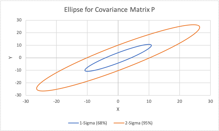
In Figure 7, you will see the covariance matrix, P, that was used to create these error ellipses. Three key takeaways from these figures are:
- The size of the ellipses in Figure 4 and Figure 6 are the same but the covariance matrices look different because Figure 6 has rotated ellipses.
- Figure 6 and Figure 7 variance terms do not align with the magnitude of the semi-major and semi-minor axes (i.e. a and b) as they did when the data was not correlated. This again is due to the rotation.
- The cross terms (i.e. sigma xy) are non-zero because there is correlation between x and y. The angle of rotation for Figure 6 and Figure 7 is 45 degrees.

How to Use Ellipses when Designing a Kalman Filter
When designing a Kalman Filter, covariance matrices are constantly being updated. This means that the error is growing and shrinking and changing.
Enjoying the article? If you’re thinking about getting a Capital One card, using this referral link helps support the site at no extra cost to you. Thanks!
Most likely your goal is to minimize the error of the system state you are estimating. By plotting this ellipse for your covariance matrix or parts of your covariance matrix, it can help you intuitively see how your filter is working and whether its performing in the way you thought.
How to Plot a Confidence Ellipse
In order to plot a confidence ellipse based on your covariance matrix, you need to identify the defining characteristics of a confidence ellipse: confidence interval e.g. 95%, major axis length, minor axis length, angle of rotation, and center of the ellipse. As described above, these can be determined by the covariance matrix.
There are multiple ways in which you can determine these characteristics but the simplest is by using some linear algebra. Conveniently, the eigenvalues represent the major and minor axes, and the eigenvectors represent the directional vectors of the major and minor axis. Using some trigonometry, you can determine the rotation angle of the error ellipse with the eigenvectors.
The confidence interval is based on the chi square value for the confidence interval you are plotting. The major and minor axis are determined by the eigenvalues of the matrix. And the angle of rotation is determined from the eigenvectors of the covariance matrix.
Dear Mr. Franklin,
I hope this message finds you well. Congratulations on your insightful post regarding the representation of covariance matrices. You have highlighted some intriguing properties that can be derived from them.
I am looking forward to seeing you expand your article to include the equations for calculating the ellipse parameters from the elements of a 2×2 covariance matrix, as well as the equations for deriving a 3×3 covariance matrix that leads to an error ellipsoid. For additional insights, I would recommend referring to the following open-access article: [1].
Moreover, I noticed that Figures 1 and 2 are related, and to enhance clarity, it might be beneficial to indicate the 1-sigma boundaries (the “standard”) in Figure 1, as already depicted in Figure 2. Figure 2 accurately represents the 1D Normal Distribution with a 95% Confidence Interval area. Given that the 1-sigma and 2-sigma regions differ by an expansion factor, it would be helpful to note that the area under the curve increases when plotting the 2-sigma (95% confidence level or 5% significance level) curve.
Thank you for your valuable contribution to this topic!
Best regards,
gps
—
Reference:
[1] Linkwitz, K. (1988). Einige Bemerkungen zur Fehlerellipse und zum Fehlerellipsoid. E-Periodica, 86. DOI: https://doi.org/10.5169/seals-233771