What is the Extended Kalman Filter?
The Extended Kalman Filter is a special Kalman Filter used when working with nonlinear systems. Since the Kalman Filter can not be applied to nonlinear systems, the Extended Kalman Filter was created to solve that problem. Specifically, it was used in the development of navigation control systems aboard Apollo 11. And like many other real world systems, the behavior is not linear so a traditional Kalman Filter can not be used. This post will walk you through an Extended Kalman Filter Python example so you can see how one can be implemented!
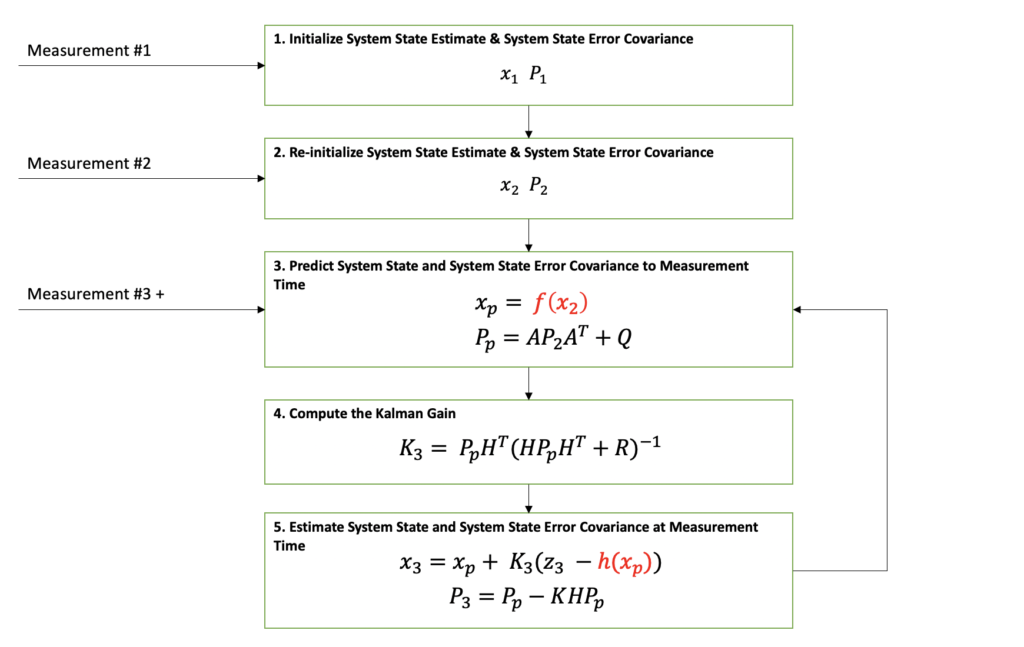
In the diagram below, it can be seen that the Extended Kalman Filter’s general flow is exactly the same as the Kalman Filter. The main two differences between the Kalman Filter and the Extended Kalman Filter are represented in red font. In addition to these differences, there are some lower level differences that I will cover in more detail below.
This article assumes that the reader understands the core concepts of the Kalman Filter. If you want a refresher before reading on, try skimming my Kalman Filter Explained Simply article.
Python Example Overview
The Extended Kalman Filter Python example chosen for this article takes in measurements from a ground based radar tracking a ship in a harbor and estimates the ships position and velocity. The radar measurements are in a local polar coordinate frame and the filter’s state estimate is in a local cartesian coordinate frame. The measurement to state estimate relationship i.e. polar to cartesian is nonlinear.
In this example, the ship is traveling in a straight line at constant velocity of 20 meters/sec or about 45 miles per hour. It is located about 3250 meters away or about 2 miles. The measurements are being reported at 1 hertz or once per second. The measurements are being reported as the range and azimuth values in local polar frame and input measurement data can be seen in the two plots below.
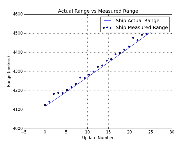
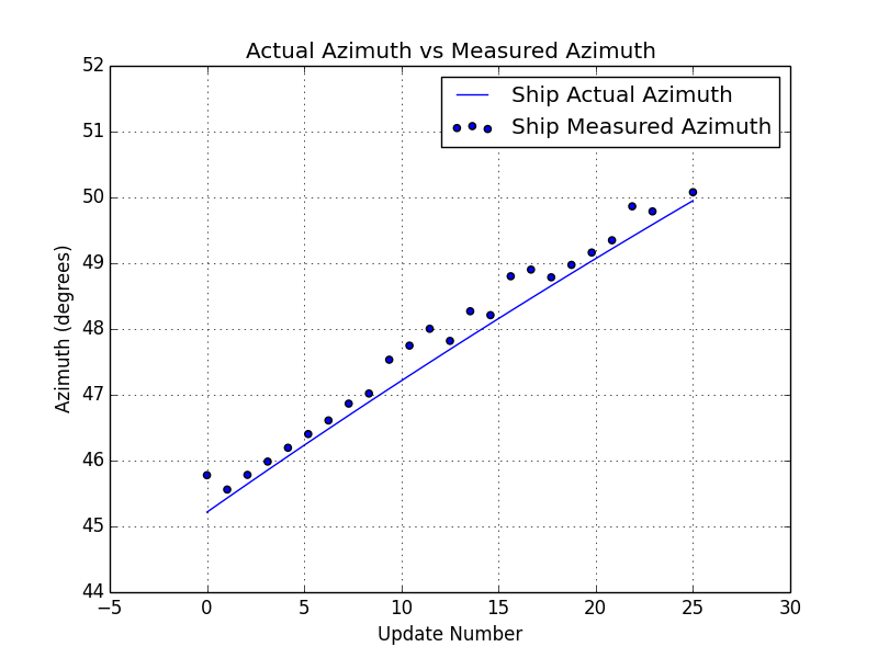
A simulation technique was used to generate these measurements. The code for simulating this ship behavior is beyond the scope of this post, but the plots above show the noisy measurements that are based on simulated position data.
On the Initialization of the Extended Kalman Filter
As can be seen in the Extended Kalman Filter diagram above, the first two measurements are needed before filtering can be begin. The reason for this is because the output state estimate needs to be initialized. There are different approaches to filter initialization based on your application but for this example, the first two position measurements will be used to form the state estimate which consists of the position and velocity.
Logically, one can make sense of this. The first position measurement received only tells you about the ships position at one point in time. Only after you receive the second measurement, can you compute a velocity i.e. change in position measurement divided by the time difference between the two measurements.
Extended Kalman Filter Python Example
Let’s take a look at the input, output, and system model equations before we dive into the code. This should make reading the code much easier.
Input and Output Equations
As mentioned above, the input measurements for this Extended Kalman Filter Python example are in the local polar coordinate frame. And these are the equations that represent these measurements.

z is the measurement vector, R is the measurement covariance matrix and t is the time at which the measurement was taken. m is used as a subscript to indicate measurements.
The above input measurements are filtered and a system state estimate is computed and output in the following form.

x is the state vector, P is the state covariance matrix, and T is the time at which the state estimate is valid. In this example, this time will reflect the last measurement time that was used to compute the state estimate.
System Model Equations for Prediction Step
As mentioned above, the system model equations are where the primary differences between the Extended Kalman Filter and the traditional Kalman Filter lie. For this example, the A and Q matrices used are not any different than matrices that would be used in a Kalman Filter. Those equations are the following.

The A matrix above is the state transition matrix. This matrix is used to extrapolate the state vector and state covariance from the last data time to align with the data time of the new measurement. This matrix was developed assuming the ship was traveling linearly at constant velocity i.e. using physics equations of motion.
The Q matrix is the system noise matrix. This represents the uncertainty in the system prediction model. For this example, the A matrix assumes the ship is traveling in a linear motion at a constant velocity. But in reality, this is not always true. The Q matrix is used to add error to the state estimate prediction to account for those differences in linear motion and small accelerations or decelerations. The values used in this example are not optimized. Optimization of these parameters is outside the scope of this post.
Here are the prediction equations from Step 3 in the diagram above.

System Model Equations for Estimation Step
The estimation process for the Extended Kalman Filter is performed in two steps. First, the Kalman Gain is computed. Second, the state vector and state covariance for the new measurement time is computed with the Kalman Gain. Both of these steps require the use of an H matrix. The H matrix is the state-to-measurement transition matrix. This matrix is used to transform the predicted state vector and covariance matrix into the same form as the input measurement. For this Extended Kalman Filter example, the state and measurement relationship is nonlinear. Because of this nonlinear relationship, the H matrix is different than that of a traditional Kalman Filter. Specifically, the H matrix is a jacobian matrix. The derivation and applications of the jacobian matrix are outside the scope of this post. The important features to note about the jacobian at this time is that is made up of first order partial differential equations. Here is the H matrix for this example.

The partial differential equations were computed with the following polar to cartesian relationships for range and azimuth.

After the H matrix is computed, the Kalman Gain can be computed. The Kalman Gain equations that follow consist of two steps. First, compute the innovation matrix, S. Then compute the gain, K.

The estimation steps use the Kalman Gain, K. The estimation steps include estimating the new system state as well as the associated state covariance matrix. One difference you can see in these equations compared to the traditional Kalman Filter estimation equations, is the h(xP) function. This function represents the state-to-measurement nonlinear transformation.

h(xP) is defined by the equation below for this example. These equations should look familiar because these are the same equations used to compute the jacobian H matrix.

Our Extended Kalman Filter tutorial is implemented in Python with these equations. Next, we will review the implementation details with code snippets and comments.
Python Implementation for the Extended Kalman Filter Example
In order to develop and tune a Python Extended Kalman Filter, you need the following source code functionality:
- Input measurement data (real or simulated)
- Extended Kalman Filter algorithm
- Data collection and visualization tools
- Test code to read in measurement data, execute filter logic, collect data, and plot the collected data
For this tutorial, multiple Python libraries are used to accomplish the above functionality. The NumPy Python library is used for arrays, matrices, and linear algebra operations on those structures. The Matplotlib is used to plot input and output data. Assuming these packages are installed, this is the code used to import and assign a variable name to these packages.
import numpy as np
from numpy.linalg import inv
import matplotlib.pyplot as plt
Extended Kalman Filter Algorithm
The algorithm is implemented using one function with two input arguments, the measurement data structure, z, and the update number, updateNumber. The update number is not a necessary input variable. But for this example, it was easier to implement. Additionally, the update number was used as the time stamp for each measurement because the measurements were reported once a second. I will update this in the future to be more robust.
There are three main processing threads through this function determined by the update number: initialization, re-initialization, and filtering. Here is the code:
def ekfilter(z, updateNumber):
    dt = 1.0
    j = updateNumber

    # Initialize State
    if updateNumber == 0: # First Update

        # compute position values from measurements
        # x = r*sin(b)
        temp_x = z[0][j]*np.sin(z[1][j]*np.pi/180)
        # y = r*cos(b)
        temp_y = z[0][j]*np.cos(z[1][j]*np.pi/180)

        # state vector
        # - initialize position values
        ekfilter.x = np.array([[temp_x],
                            [temp_y],
                            [0],
                            [0]])

        # state covariance matrix
        # - initialized to zero for first update
        ekfilter.P = np.array([[0, 0, 0, 0],
                                 [0, 0, 0, 0],
                                 [0, 0, 0, 0],
                                 [0, 0, 0, 0]])

        # state transistion matrix
        # - linear extrapolation assuming constant velocity
        ekfilter.A = np.array([[1, 0, dt, 0],
                             [0, 1, 0, dt],
                             [0, 0, 1, 0],
                             [0, 0, 0, 1]])


        # measurement covariance matrix
        ekfilter.R = z[2][j]

        # system error matrix
        # - initialized to zero matrix for first update
        ekfilter.Q = np.array([[0, 0, 0, 0],
                                 [0, 0, 0, 0],
                                 [0, 0, 0, 0],
                                 [0, 0, 0, 0]])

        # residual and kalman gain
        # - not computed for first update
        # - but initialized so it could be output
        residual = np.array([[0, 0],
                      [0, 0]])
        K = np.array([[0, 0],
                      [0, 0],
                      [0, 0],
                      [0, 0]])

    # Reinitialize State
    if updateNumber == 1: # Second Update

        prev_x = ekfilter.x[0][0]
        prev_y = ekfilter.x[1][0]


        # x = r*sin(b)
        temp_x = z[0][j]*np.sin(z[1][j]*np.pi/180)
        # y = r*cos(b)
        temp_y = z[0][j]*np.cos(z[1][j]*np.pi/180)
        temp_xv = (temp_x - prev_x)/dt
        temp_yv = (temp_y - prev_y)/dt

        # state vector
        # - reinitialized with new position and computed velocity
        ekfilter.x = np.array([[temp_x],
                            [temp_y],
                            [temp_xv],
                            [temp_yv]])

        # state covariance matrix
        # - initialized to large values
        # - more accurate position values can be used based on measurement
        #   covariance but this example does not go that far
        ekfilter.P = np.array([[100, 0, 0, 0],
                                 [0, 100, 0, 0],
                                 [0, 0, 250, 0],
                                 [0, 0, 0, 250]])

        # state transistion matrix
        # - linear extrapolation assuming constant velocity
        ekfilter.A = np.array([[1, 0, dt, 0],
                             [0, 1, 0, dt],
                             [0, 0, 1, 0],
                             [0, 0, 0, 1]])

        # measurement covariance matrix
        # - provided by the measurment source
        ekfilter.R = z[2][j]

        # system error matrix
        # - adds 4.5 meter std dev in x and y position to state covariance
        # - adds 2 meters per second std dev in x and y velocity to state covariance
        # - these values are not optimized but work for this example
        ekfilter.Q = np.array([[20, 0, 0, 0],
                                 [0, 20, 0, 0],
                                 [0, 0, 4, 0],
                                 [0, 0, 0, 4]])
        # residual and kalman gain
        # - not computed for first update
        # - but initialized so it could be output
        residual = np.array([[0, 0],
                      [0, 0]])
        K = np.array([[0, 0],
                      [0, 0],
                      [0, 0],
                      [0, 0]])
    if updateNumber > 1: # Third + Updates

      # Predict State Forward
      x_prime = ekfilter.A.dot(ekfilter.x)

      # Predict Covariance Forward
      P_prime = ekfilter.A.dot(ekfilter.P).dot(ekfilter.A.T) + ekfilter.Q

      # state to measurement transition matrix
      x1 = x_prime[0][0]
      y1 = x_prime[1][0]
      x_sq = x1*x1
      y_sq = y1*y1
      den = x_sq+y_sq
      den1 = np.sqrt(den)
      ekfilter.H = np.array([[  x1/den1,    y1/den1, 0, 0],
                           [y1/den, -x1/den, 0, 0]])

      ekfilter.HT = np.array([[x1/den1, y1/den],
                              [y1/den1, -x1/den],
                              [0, 0],
                              [0, 0]])

      # measurement covariance matrix
      ekfilter.R = z[2][j]

      # Compute Kalman Gain
      S = ekfilter.H.dot(P_prime).dot(ekfilter.HT) + ekfilter.R
      K = P_prime.dot(ekfilter.HT).dot(np.linalg.inv(S))

      # Estimate State
      # temp_z = current measurement in range and azimuth
      temp_z = np.array([[z[0][j]],
                         [z[1][j]]])

      # compute the predicted range and azimuth
      # convert the predicted cartesian state to polar range and azimuth
      pred_x = x_prime[0][0]
      pred_y = x_prime[1][0]

      sumSquares = pred_x*pred_x + pred_y*pred_y
      pred_r = np.sqrt(sumSquares)
      pred_b = np.arctan2(pred_x, pred_y) * 180/np.pi
      h_small = np.array([[pred_r],
                       [pred_b]])

      # compute the residual
      # - the difference between the state and measurement for that data time
      residual = temp_z - h_small

      # Compute new estimate for state vector using the Kalman Gain
      ekfilter.x = x_prime + K.dot(residual)

      # Compute new estimate for state covariance using the Kalman Gain
      ekfilter.P = P_prime - K.dot(ekfilter.H).dot(P_prime)

    return [ekfilter.x[0], ekfilter.x[1], ekfilter.x[2], ekfilter.x[3], ekfilter.P, K, residual, updateNumber];
# End of ekfilter
Testing the Extended Kalman Filter Algorithm
In order to test this algorithm implementation, real data or simulated data is needed. For this tutorial, simulated data is generated and used to test the algorithm. As mentioned above, the simulation for this example is outside the scope of this post. More information on how to simulate inputs can be found in my Kalman Filter Made Easy Book. Available in print and eBook!
The test code below was used to test this algorithm. The getMeasurements() function returns an array of arrays of measurement information in the following form: [measurement_range, meas_azimuth, measurement_cov, meas_time]
z = getMeasurements()
for iii in range(0, len(z[0])):
  # for each measurement, call the Extended Kalman Filter function
  f = ekfilter(z, iii)
Filter Results and Analysis
There are many different ways to analyze your filter’s performance. And every application will require different analysis because each will have its own performance requirements. Here are two plots that helped us understand if this filter was working.
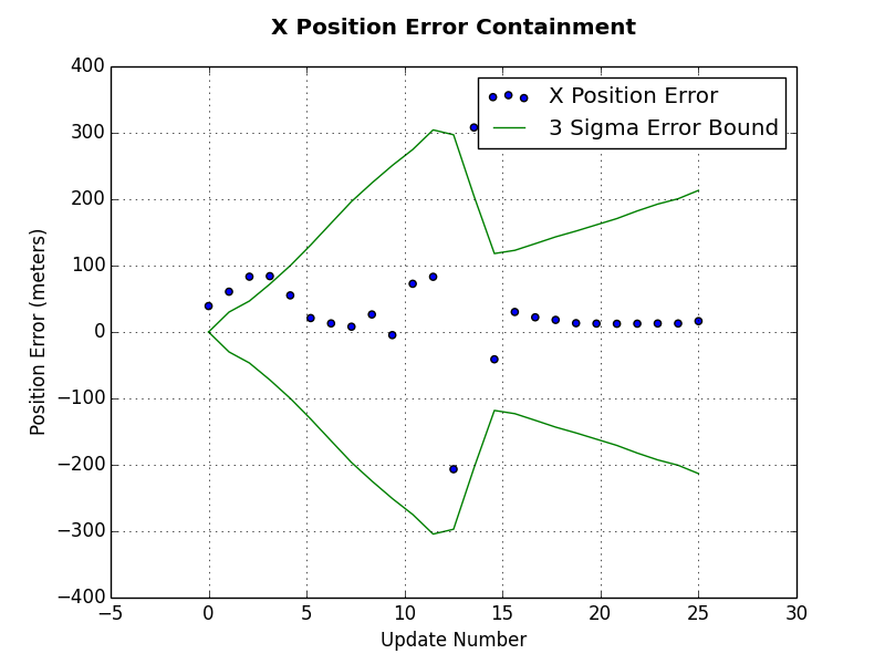
The first plot is an error plot for the x position estimate. This plot includes the x position error, which is computed as the x position estimate minus the real x position that was used to generate the polar measurement. In addition to the x position error, the green lines represent the estimated error bounds computed from the state covariance estimate. You can see in this plot that sometimes the x position error falls outside the error bounds. Again, based on your application requirements, this may or may not be okay. The x position error starts to settle within the error bounds after update number 15.
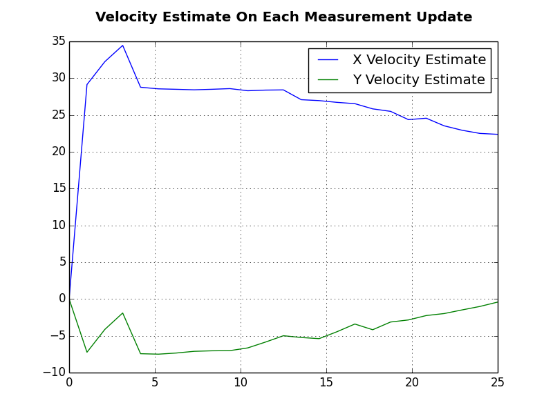
Another plot used was the estimated velocity for the ship. It can be seen that the x and y velocity values vary during the first few updates but then begin to settle at the actual values used for measurement generation i.e. x velocity at 20 meters per second and y velocity at 0 meters per second. This is a good sign that the filter is working because it is able to accurately estimate the ships velocity based only on position measurements in a different coordinate frame.
Extended Kalman Filters can diverge. This means that the filter’s estimate will grow uncontrollably and won’t represent the true system state. Researchers continue to conduct research to find ways to correct that divergence. Divergence correction is outside the scope of this post.
Summary
I wish you the best of luck in your filtering work as you move forward on your projects! Please leave a comment if you enjoyed this post! If you enjoyed reading this post, check out my book Kalman Filter Made Easy. and my other book Unscented Kalman Filter Made Easy. These books (and eBooks) will go into more details about simulation, analysis, and visualization of the Kalman Filter, Extended Kalman Filter, and the Unscented Kalman Filter.